Example: A Real-Valued Multi-Objective Optimization Problem
Below is a simple two-variable multi-objective problem to illustrate real-valued optimization with pymoors. We have two continuous decision variables, \(x_1\) and \(x_2\), both within a given range. We define two objective functions to be minimized simultaneously, and we solve this using the popular NSGA2 algorithm.
Mathematical Formulation
Let \(\mathbf{x} = (x_1, x_2)\) be our decision variables, each constrained to the interval \([-2, 2]\). We define the following objectives:
Interpretation
- \(f_1\) measures the distance of \(\mathbf{x}\) from the origin \((0,0)\) in the 2D plane.
- \(f_2\) measures the distance of \(\mathbf{x}\) from the point \((1,0)\).
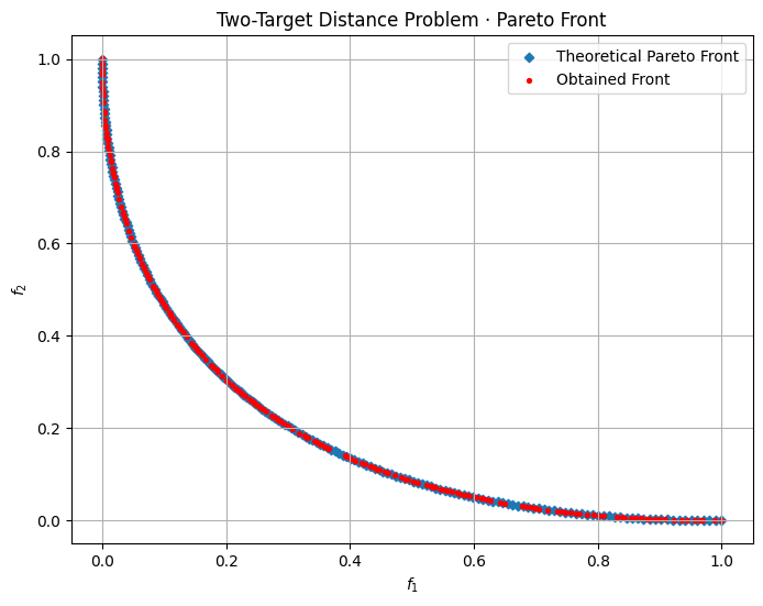
Thus, \(\mathbf{x}\) must compromise between being close to \((0,0)\) and being close to \((1,0)\). There is no single point in \([-2,2]^2\) that simultaneously minimizes both distances perfectly (other than at the boundary of these trade-offs), so we end up with a Pareto front rather than a single best solution.
:dep ndarray = "*"
:dep moors = "0.2.6"
:dep plotters = "0.3.6"

use ndarray::{Array2, Ix2};
use moors::{
    NoConstraints,
    algorithms::Nsga2Builder,
    duplicates::CloseDuplicatesCleaner,
    operators::{GaussianMutation, SimulatedBinaryCrossover, RandomSamplingFloat},
    genetic::Population
};
use plotters::prelude::*;

// General: compute two-objective fitness (squared distances).
fn fitness_fn(genes: &Array2<f64>) -> Array2<f64> {
    let n = genes.nrows();
    let mut result = Array2::<f64>::zeros((n, 2));

    let x1 = genes.column(0);
    let x2 = genes.column(1);

    let f1 = &x1.mapv(|v| v.powi(2)) + &x2.mapv(|v| v.powi(2));
    let f2 = &x1.mapv(|v| (v - 1.0).powi(2)) + &x2.mapv(|v| v.powi(2));

    result.column_mut(0).assign(&f1);
    result.column_mut(1).assign(&f2);
    result
}

// General: run NSGA-II and collect population.
let population: Population<Ix2, Ix2> = {
    let mut algorithm = Nsga2Builder::default()
        .sampler(RandomSamplingFloat::new(-2.0, 2.0))
        .crossover(SimulatedBinaryCrossover::new(15.0))
        .mutation(GaussianMutation::new(0.1, 0.01))
        .duplicates_cleaner(CloseDuplicatesCleaner::new(1e-16))
        .fitness_fn(fitness_fn)
        .constraints_fn(NoConstraints)
        .num_vars(2)
        .population_size(200)
        .num_offsprings(200)
        .num_iterations(100)
        .mutation_rate(0.2)
        .crossover_rate(0.9)
        .keep_infeasible(false)
        .verbose(false)
        .seed(42)
        .build()
        .unwrap();

    algorithm.run().expect("NSGA2 run failed");
    algorithm.population.unwrap().clone()
};

// General: theoretical Pareto front curve.
let n = 200usize;
let t: Vec<f64> = (0..n).map(|i| i as f64 / (n as f64 - 1.0)).collect();
let f1_theo: Vec<f64> = t.iter().map(|&x| x * x).collect();
let f2_theo: Vec<f64> = t.iter().map(|&x| (x - 1.0).powi(2)).collect();

// General: obtained front from the algorithm.
let fitness = population.fitness;
let f1: Vec<f64> = fitness.column(0).to_vec();
let f2: Vec<f64> = fitness.column(1).to_vec();

// General: define axes with headroom.
let mut x_max = f1.iter().copied().chain(f1_theo.iter().copied()).fold(0.0_f64, f64::max);
let mut y_max = f2.iter().copied().chain(f2_theo.iter().copied()).fold(0.0_f64, f64::max);
x_max = (x_max * 1.05).max(1.0);
y_max = (y_max * 1.05).max(1.0);

// General: render to in-memory SVG and emit as rich output (no files).
let mut svg = String::new();
{
    let backend = SVGBackend::with_string(&mut svg, (800, 600));
    let root = backend.into_drawing_area();
    root.fill(&WHITE).unwrap();

    let mut chart = ChartBuilder::on(&root)
        .caption("Two-Target Distance Problem · Pareto Front", ("DejaVu Sans", 22))
        .margin(10)
        .x_label_area_size(40)
        .y_label_area_size(60)
        .build_cartesian_2d(0f64..x_max, 0f64..y_max)
        .unwrap();

    chart.configure_mesh()
        .x_desc("f1")
        .y_desc("f2")
        .axis_desc_style(("DejaVu Sans", 14))
        .light_line_style(&RGBColor(220, 220, 220))
        .draw()
        .unwrap();

    chart.draw_series(
        f1_theo.iter().zip(f2_theo.iter()).map(|(&x, &y)| {
            Circle::new((x, y), 5, RGBColor(31, 119, 180).filled())
        })
    ).unwrap()
     .label("Theoretical Pareto Front")
     .legend(|(x, y)| Circle::new((x, y), 5, RGBColor(31, 119, 180).filled()));

    chart.draw_series(
        f1.iter().zip(f2.iter()).map(|(&x, &y)| {
            Circle::new((x, y), 3, RGBColor(255, 0, 0).filled())
        })
    ).unwrap()
     .label("Obtained Front")
     .legend(|(x, y)| Circle::new((x, y), 3, RGBColor(255, 0, 0).filled()));

    chart.configure_series_labels()
        .border_style(&RGBAColor(0, 0, 0, 0.3))
        .background_style(&WHITE.mix(0.9))
        .label_font(("DejaVu Sans", 13))
        .draw()
        .unwrap();

    root.present().unwrap();
}

println!("EVCXR_BEGIN_CONTENT image/svg+xml\n{}\nEVCXR_END_CONTENT", svg);

import numpy as np
import matplotlib.pyplot as plt

from pymoors import (
    Nsga2,
    RandomSamplingFloat,
    GaussianMutation,
    SimulatedBinaryCrossover,
    CloseDuplicatesCleaner,
    Constraints
)
from pymoors.typing import TwoDArray


def fitness(genes: TwoDArray) -> TwoDArray:
    x1 = genes[:, 0]
    x2 = genes[:, 1]
    # Objective 1: Distance to (0,0)
    f1 = x1**2 + x2**2
    # Objective 2: Distance to (1,0)
    f2 = (x1 - 1) ** 2 + x2**2
    # Combine the two objectives into a single array
    return np.column_stack([f1, f2])


algorithm = Nsga2(
    sampler=RandomSamplingFloat(min=-2, max=2),
    crossover=SimulatedBinaryCrossover(distribution_index=15),
    mutation=GaussianMutation(gene_mutation_rate=0.1, sigma=0.01),
    fitness_fn=fitness,
    constraints_fn = Constraints(lower_bound = -2.0, upper_bound = 2.0),
    duplicates_cleaner=CloseDuplicatesCleaner(epsilon=1e-16),
    num_vars=2,
    population_size=200,
    num_offsprings=200,
    num_iterations=100,
    mutation_rate=0.2,
    crossover_rate=0.9,
    keep_infeasible=False,
    seed=42,
    verbose=False,
)

algorithm.run()
population = algorithm.population

# Plot the results
t = np.linspace(0.0, 1.0, 200)
f1_theo = t**2
f2_theo = (t - 1.0) ** 2


plt.figure(figsize=(8, 6))
plt.scatter(f1_theo, f2_theo, marker="D", s=18, label="Theoretical Pareto Front")
plt.scatter(
    population.fitness[:, 0],
    population.fitness[:, 1],
    c="r",
    s=8,
    marker="o",
    label="Obtained Front",
)
plt.xlabel("$f_1$")
plt.ylabel("$f_2$")
plt.title("Two-Target Distance Problem · Pareto Front")
plt.grid(True)
plt.legend()
plt.show()