RNSGA-II

RNSGA-II is an advanced, elitist multiobjective evolutionary algorithm that extends NSGA-II by incorporating reference points to guide the search toward regions of interest specified by the decision-maker. This modification is introduced in the survival selection phase, where the algorithm not only considers Pareto dominance and crowding distance but also evaluates the proximity of each solution to predefined reference points.

Key Features

Fast Nondominated Sorting: RNSGA-II sorts the population based on Pareto dominance with a computational complexity of \(O(MN^2)\), where \(M\) is the number of objectives and \(N\) is the population size.
Elitist Selection with Reference Points: The algorithm forms a combined pool of parent and offspring populations. From this pool, the best solutions are selected not only based on fitness and diversity but also on their proximity to the reference points. This ensures that solutions closer to the preferred regions have a higher chance of survival.
Crowding Distance for Diversity Maintenance: To maintain a diverse Pareto front, RNSGA-II computes the crowding distance for each individual. In addition, it assesses each solution’s distance from the reference points.

Individuals with a larger crowding distance or those nearer to the reference points are favored, thus promoting diversity while also focusing the search in regions of interest.

Modified Survival Selection: The survival selection process in RNSGA-II is enhanced by:
Reference Point Proximity: Evaluating how close each solution is to the predefined reference points.
Combined Ranking: First ranking solutions by Pareto dominance, then by crowding distance, and finally giving extra priority to those closer to the reference points. This approach effectively balances convergence toward the Pareto-optimal front with targeted exploration of preferred regions.
Constraint Handling: When constraints_fn are present, feasible solutions are always favored. Among these, solutions with a better (i.e., lower) nondomination rank are preferred, and if ties occur, those with a higher crowding distance and closer to the reference points are selected.

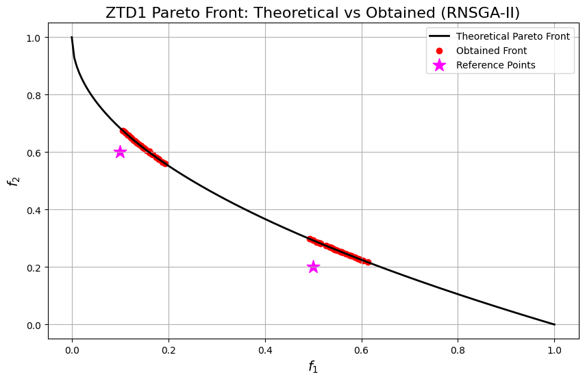
ZTD1 Problem

The ZTD1 problem is commonly used as a benchmark problem to evaluate multiobjective optimization algorithms that incorporate reference points. It challenges the algorithm with:

Two Conflicting Objectives:
\(f_1(\mathbf{x}) = x_1\)
\(f_2(\mathbf{x}) = g(\mathbf{x}) \cdot h(f_1(\mathbf{x}), g(\mathbf{x}))\)
Auxiliary Functions:
\(g(\mathbf{x}) = 1 + \frac{9}{n-1}\sum_{i=2}^{n} x_i\)
\(h(f_1, g) = 1 - \sqrt{\frac{f_1}{g}}\)
Key Characteristics:
Continuous and Convex Pareto Front: Unlike problems with discontinuous fronts, ZTD1 features a continuous and convex Pareto front. This facilitates convergence while still posing a challenge in maintaining solution diversity.
Incorporation of Reference Points: The use of reference points in RNSGA-II directs the search toward specific regions of the Pareto front, ensuring that the obtained solutions align with the decision-maker’s preferences.

Domain: Each decision variable \(x_i\) is typically within the interval \([0, 1]\), and the problem is commonly defined with \(n = 30\) variables.

RustPython

:dep ndarray = "*"
:dep moors = "*"
:dep plotters = "0.3.6"

use ndarray::{s, array, Array2, Axis, Ix2};
use moors::{
    impl_constraints_fn,
    algorithms::Rnsga2Builder,
    duplicates::CloseDuplicatesCleaner,
    operators::{GaussianMutation, RandomSamplingFloat, ExponentialCrossover, Rnsga2ReferencePointsSurvival},
    genetic::Population,
};
use plotters::prelude::*

/// Evaluate the ZTD1 objectives in a fully vectorized manner.
fn evaluate_ztd1(x: &Array2<f64>) -> Array2<f64> {
    let n = x.nrows();
    let m = x.ncols();

    // clamp to [0,1] to mirror the Python domain constraints
    let clamped = x.mapv(|v| v.clamp(0.0, 1.0));

    let f1 = clamped.column(0).to_owned();
    let tail = clamped.slice(s![.., 1..]);
    let sums = tail.sum_axis(Axis(1));
    let g = sums.mapv(|s| 1.0 + 9.0 / ((m as f64) - 1.0) * s);
    let ratio = &f1 / &g;
    let f2 = &g * (1.0 - ratio.mapv(|r| r.sqrt()));

    let mut out = Array2::<f64>::zeros((n, 2));
    out.column_mut(0).assign(&f1);
    out.column_mut(1).assign(&f2);
    out
}

/// Compute the theoretical Pareto front for ZTD1.
fn ztd1_theoretical_front() -> (Vec<f64>, Vec<f64>) {
    let mut f1_theo = Vec::with_capacity(200);
    let mut f2_theo = Vec::with_capacity(200);
    for i in 0..200 {
        let v = i as f64 / 199.0;
        f1_theo.push(v);
        f2_theo.push(1.0 - v.sqrt());
    }
    (f1_theo, f2_theo)
}

// Create constraints using the macro impl_constraints_fn
impl_constraints_fn!(BoundConstraints, lower_bound = 0.0, upper_bound = 1.0);



// Set up RNSGA-II algorithm with epsilon = 0.005
let population: Population<Ix2, Ix2> = {
    // Define two reference points (for example, points on the Pareto front)
    let rp: Array2<f64> = array![[0.5, 0.2], [0.1, 0.6]];
    let epsilon = 0.005;
    let survivor = Rnsga2ReferencePointsSurvival::new(rp, epsilon);
    let mut algorithm = Rnsga2Builder::default()
        .sampler(RandomSamplingFloat::new(0.0, 1.0))
        .crossover(ExponentialCrossover::new(0.75))
        .mutation(GaussianMutation::new(0.1, 0.01))
        .survivor(survivor)
        .fitness_fn(evaluate_ztd1)
        .constraints_fn(BoundConstraints)
        .duplicates_cleaner(CloseDuplicatesCleaner::new(1e-8))
        .num_vars(30)
        .population_size(50)
        .num_offsprings(50)
        .num_iterations(700)
        .mutation_rate(0.1)
        .crossover_rate(0.9)
        .keep_infeasible(false)
        .verbose(false)
        .seed(1729)
        .build()
        .expect("Failed to build RNSGA-II");

    // Run the algorithm
    algorithm.run().expect("RNSGA2 run failed");
    algorithm.population().unwrap().clone()
};

// Compute the theoretical Pareto front for ZTD1
let (f1_theo, f2_theo) = ztd1_theoretical_front();

// Get the best Pareto front obtained (as a Population instance)
let fitness = population.fitness;

// Extract the obtained fitness values (each row is [f1, f2])
let f1_found: Vec<f64> = fitness.column(0).to_vec();
let f2_found: Vec<f64> = fitness.column(1).to_vec();

// Compute the theoretical Pareto front for ZTD1
let (f1_theo, f2_theo) = ztd1_theoretical_front();

// Plot the theoretical Pareto front, obtained front, and reference points
let mut svg = String::new();
{
    let backend = SVGBackend::with_string(&mut svg, (1000, 600));
    let root = backend.into_drawing_area();
    root.fill(&WHITE).unwrap();

    let grid_color = RGBColor(220, 220, 220);

    // Build axis ranges with headroom including reference points
    let reference_points: Vec<[f64; 2]> = vec![[0.5, 0.2], [0.1, 0.6]];

    // Compute min/max from actual data
    let (mut x_min, mut x_max) = (f1_theo[0], f1_theo[0]);
    let (mut y_min, mut y_max) = (f2_theo[0], f2_theo[0]);

    for &x in f1_theo.iter().chain(f1_found.iter()) {
        if x < x_min { x_min = x; }
        if x > x_max { x_max = x; }
    }
    for &y in f2_theo.iter().chain(f2_found.iter()) {
        if y < y_min { y_min = y; }
        if y > y_max { y_max = y; }
    }

    // Add a small margin (5%)
    let xr = (x_max - x_min);
    let yr = (y_max - y_min);
    x_min -= xr * 0.05;
    x_max += xr * 0.05;
    y_min -= yr * 0.05;
    y_max += yr * 0.05;

    let mut chart = ChartBuilder::on(&root)
        .caption("ZDT1 Pareto Front: Theoretical vs Obtained (R-NSGA-II)", ("DejaVu Sans", 22))
        .margin(10)
        .x_label_area_size(40)
        .y_label_area_size(60)
        .build_cartesian_2d(x_min..x_max, y_min..y_max)
        .unwrap();

    chart.configure_mesh()
        .x_desc("f1")                      // plt.xlabel("$f_1$")
        .y_desc("f2")                      // plt.ylabel("$f_2$")
        .axis_desc_style(("DejaVu Sans", 14))
        .light_line_style(&grid_color)     // plt.grid(True)
        .draw()
        .unwrap();

    // Theoretical Pareto Front (black solid line, linewidth=2)
    chart.draw_series(LineSeries::new(
        f1_theo.iter().cloned().zip(f2_theo.iter().cloned()),
        ShapeStyle {
            color: BLACK.to_rgba(),
            filled: false,
            stroke_width: 2,
        },
    )).unwrap()
     .label("Theoretical Pareto Front")
     .legend(|(x, y)| PathElement::new(vec![(x - 10, y), (x + 10, y)], &BLACK));

    // Obtained Front (red circles)
    chart.draw_series(
        f1_found.iter().zip(f2_found.iter()).map(|(&x, &y)| {
            Circle::new((x, y), 3, RGBColor(255, 0, 0).filled())
        })
    ).unwrap()
     .label("Obtained Front")
     .legend(|(x, y)| Circle::new((x, y), 4, RGBColor(255, 0, 0).filled()));

    // Reference Points
    chart.draw_series(
        reference_points.iter().map(|p| {
            TriangleMarker::new((p[0], p[1]), 8, MAGENTA.filled())
        })
    ).unwrap()
     .label("Reference Points")
     .legend(|(x, y)| TriangleMarker::new((x, y), 8, MAGENTA.filled()));

    chart.configure_series_labels()
        .border_style(&BLACK.mix(0.3))
        .background_style(&WHITE.mix(0.9))
        .label_font(("DejaVu Sans", 13))
        .draw()
        .unwrap();

    root.present().unwrap();
}

// Emit as rich output for evcxr
println!("EVCXR_BEGIN_CONTENT image/svg+xml\n{}\nEVCXR_END_CONTENT", svg);

svg

import numpy as np
import matplotlib.pyplot as plt

from pymoors import (
    Rnsga2,
    RandomSamplingFloat,
    GaussianMutation,
    ExponentialCrossover,
    CloseDuplicatesCleaner,
    Constraints
)
from pymoors.schemas import Population
from pymoors.typing import TwoDArray

np.seterr(invalid="ignore")


def evaluate_ztd1(x: TwoDArray) -> TwoDArray:
    """
    Evaluate the ZTD1 objectives in a fully vectorized manner.
    """
    f1 = x[:, 0]
    g = 1 + 9.0 / (30 - 1) * np.sum(x[:, 1:], axis=1)
    f2 = g * (1 - np.power((f1 / g), 0.5))
    return np.column_stack((f1, f2))


def ztd1_theoretical_front():
    """
    Compute the theoretical Pareto front for ZTD1.
    """
    f1_theo = np.linspace(0, 1, 200)
    f2_theo = 1 - np.sqrt(f1_theo)
    return f1_theo, f2_theo


# Define two reference points (for example, points on the Pareto front)
reference_points = np.array([[0.5, 0.2], [0.1, 0.6]])

# Set up RNSGA-II algorithm with epsilon = 0.01
algorithm = Rnsga2(
    sampler=RandomSamplingFloat(min=0, max=1),
    crossover=ExponentialCrossover(exponential_crossover_rate=0.75),
    mutation=GaussianMutation(gene_mutation_rate=0.1, sigma=0.01),
    fitness_fn=evaluate_ztd1,
    constraints_fn=Constraints(lower_bound=0.0, upper_bound=1.0),
    duplicates_cleaner=CloseDuplicatesCleaner(epsilon=1e-8),
    num_vars=30,
    population_size=50,
    num_offsprings=50,
    num_iterations=700,
    mutation_rate=0.1,
    crossover_rate=0.9,
    keep_infeasible=False,
    reference_points=reference_points,
    verbose=False,
    epsilon=0.005,
    seed=1729,
)

# Run the algorithm
algorithm.run()

# Get the best Pareto front obtained (as a Population instance)
best: Population = algorithm.population.best_as_population
obtained_fitness = best.fitness

# Compute the theoretical Pareto front for ZTD1
f1_theo, f2_theo = ztd1_theoretical_front()

# Plot the theoretical Pareto front, obtained front, and reference points
plt.figure(figsize=(10, 6))
plt.plot(f1_theo, f2_theo, "k-", linewidth=2, label="Theoretical Pareto Front")
plt.scatter(
    obtained_fitness[:, 0],
    obtained_fitness[:, 1],
    c="r",
    marker="o",
    label="Obtained Front",
)
plt.scatter(
    [pt[0] for pt in reference_points],
    [pt[1] for pt in reference_points],
    marker="*",
    s=200,
    color="magenta",
    label="Reference Points",
)
plt.xlabel("$f_1$", fontsize=14)
plt.ylabel("$f_2$", fontsize=14)
plt.title("ZTD1 Pareto Front: Theoretical vs Obtained (RNSGA-II)", fontsize=16)
plt.legend()
plt.grid(True)
plt.show()

png