AGE-MOEA

AgeMoea is an adaptive evolutionary algorithm based on non-Euclidean geometry for many-objective optimization. Its main strength lies in discovering the geometry of the first (Pareto) front, enabling the algorithm to capture the intrinsic structure of the solution space and thereby improve both convergence and diversity.

Key Features

Adaptive Geometry-based Search: AgeMoea leverages non-Euclidean geometric principles to model the shape and curvature of the first front. This approach allows the algorithm to dynamically adjust its search strategy based on the topology and geometric structure of the optimal solutions.
Focus on Pareto Front Geometry: By emphasizing the geometry of the Pareto front, the algorithm can identify promising regions and ensure a balanced distribution of solutions along the front. This strategy favors the exploration of areas of interest while maintaining diversity.
Dynamic Evolutionary Process: Throughout its evolution, AgeMoea adapts its search parameters based on the geometric information extracted from the current solution set. This adaptive mechanism allows for more efficient navigation in complex search spaces, overcoming the limitations of traditional Euclidean metrics.

Algorithm Complexity

As stated in the referenced paper, the computational complexity of this 2 is: $$ O(M \times N^2) + O(N^3) $$ where $M$ is the number of objectives and $N$ is the population size. This complexity indicates that the algorithm may not be very efficient for large population sizes, since the $O(N^3)$ term can become computationally prohibitive as $N$ increases.

How the Algorithm Works

Non-Euclidean Metrics: Instead of relying solely on Euclidean distance, AgeMoea employs metrics that capture the true curvature and topology of the Pareto front. This distinction allows the algorithm to differentiate between solutions that are geometrically close in a traditional sense but are significantly different along the front.
Geometry-based Selection: The selection phase prioritizes solutions that best represent the geometric structure of the Pareto front. This ensures a balanced representation of diversity and an accurate depiction of the optimal front's shape.
Adaptive Parameter Tuning: As the algorithm iterates, it dynamically adjusts its parameters based on the detected geometric characteristics, enabling more effective exploration and exploitation of the solution space.

Conclusion

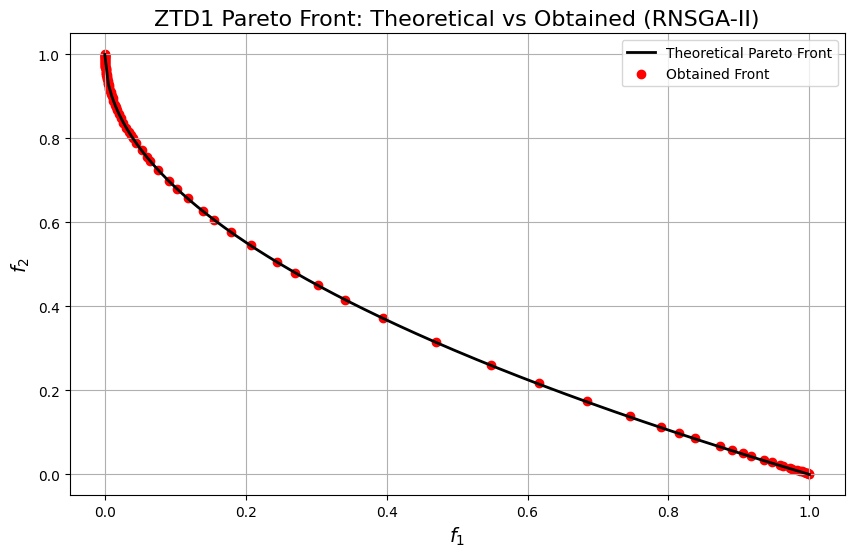
AgeMoea introduces an innovative approach to many-objective optimization by incorporating non-Euclidean geometric concepts to uncover and exploit the structure of the Pareto front. While its performance on benchmarks like ZTD1 demonstrates its ability to balance convergence and diversity, the computational complexity of $\(O(M \times N^2) + O(N^3)$\) can be a limiting factor when handling very large populations.

ZTD1 Problem

This problem was explained in the RNSGA-II section

RustPython

:dep ndarray = "*"
:dep moors = "*"
:dep plotters = "0.3.6"

use ndarray::{Array2, Axis, Ix2, s};
use moors::{
    impl_constraints_fn,
    algorithms::AgeMoeaBuilder,
    duplicates::CloseDuplicatesCleaner,
    operators::{GaussianMutation, RandomSamplingFloat, SimulatedBinaryCrossover},
    genetic::Population
};
use plotters::prelude::*;

/// Evaluate the ZDT1 objectives in a fully vectorized manner.
fn evaluate_zdt1(genes: &Array2<f64>) -> Array2<f64> {
    // First objective: f1 is simply the first column.
    let n = genes.nrows();
    let m = genes.ncols();

    let clamped = genes.mapv(|v| v.clamp(0.0, 1.0));
    let f1 = clamped.column(0).to_owned();

    // Compute g for each candidate: g = 1 + (9/(n-1)) * sum(x[1:])
    let tail = clamped.slice(s![.., 1..]);
    let sums = tail.sum_axis(Axis(1));
    let g = sums.mapv(|s| 1.0 + (9.0 / ((m as f64) - 1.0)) * s);

    // Compute the second objective: f2 = g * (1 - sqrt(f1/g))
    let ratio = &f1 / &g;
    let f2 = &g * &(1.0 - ratio.mapv(|r| r.sqrt()));

    let mut result = Array2::<f64>::zeros((n, 2));
    result.column_mut(0).assign(&f1);
    result.column_mut(1).assign(&f2);
    result
}

// Create constraints using the macro impl_constraints_fn
impl_constraints_fn!(BoundConstraints, lower_bound = 0.0, upper_bound = 1.0);

/// Compute the theoretical Pareto front for ZDT1.
fn zdt1_theoretical_front() -> (Vec<f64>, Vec<f64>) {
    let steps = 200;
    let f1_theo: Vec<f64> = (0..steps)
        .map(|i| i as f64 / (steps as f64 - 1.0))
        .collect();
    let f2_theo: Vec<f64> = f1_theo.iter().map(|&f1| 1.0 - f1.sqrt()).collect();
    (f1_theo, f2_theo)
}

// Set up AgeMoea algorithm
let population: Population<Ix2, Ix2> = {
    let mut algorithm = AgeMoeaBuilder::default()
        .sampler(RandomSamplingFloat::new(0.0, 1.0))
        .crossover(SimulatedBinaryCrossover::new(15.0))
        .mutation(GaussianMutation::new(0.1, 0.01))
        .duplicates_cleaner(CloseDuplicatesCleaner::new(1e-8))
        .fitness_fn(evaluate_zdt1)
        .constraints_fn(BoundConstraints)
        .num_vars(30)
        .population_size(100)
        .num_offsprings(100)
        .num_iterations(200)
        .mutation_rate(0.1)
        .crossover_rate(0.9)
        .keep_infeasible(false)
        .verbose(false)
        .seed(42)
        .build()
        .expect("Failed to build AgeMOEA");

    // Run the algorithm
    algorithm.run().expect("AgeMOEA run failed");
    algorithm.population().unwrap().clone()
};

// Get the best Pareto front obtained (as a Population instance)
let fitness = population.fitness;

// Extract the obtained fitness values (each row is [f1, f2])
let f1_found: Vec<f64> = fitness.column(0).to_vec();
let f2_found: Vec<f64> = fitness.column(1).to_vec();

// Compute the theoretical Pareto front for ZDT1
let (f1_theo, f2_theo) = zdt1_theoretical_front();

// Plot the theoretical Pareto front and the obtained front
let mut svg = String::new();
{
    let backend = SVGBackend::with_string(&mut svg, (1000, 700));
    let root = backend.into_drawing_area();
    root.fill(&WHITE).unwrap();

    // Compute min/max from actual data
    let (mut x_min, mut x_max) = (f1_theo[0], f1_theo[0]);
    let (mut y_min, mut y_max) = (f2_theo[0], f2_theo[0]);

    for &x in f1_theo.iter().chain(f1_found.iter()) {
        if x < x_min { x_min = x; }
        if x > x_max { x_max = x; }
    }
    for &y in f2_theo.iter().chain(f2_found.iter()) {
        if y < y_min { y_min = y; }
        if y > y_max { y_max = y; }
    }

    // Add a small margin (5%)
    let xr = (x_max - x_min);
    let yr = (y_max - y_min);
    x_min -= xr * 0.05;
    x_max += xr * 0.05;
    y_min -= yr * 0.05;
    y_max += yr * 0.05;

    let mut chart = ChartBuilder::on(&root)
        .caption("ZDT1 Pareto Front: Theoretical vs Obtained", ("DejaVu Sans", 22))
        .margin(10)
        .x_label_area_size(40)
        .y_label_area_size(60)
        .build_cartesian_2d(x_min..x_max, y_min..y_max)
        .unwrap();

    chart.configure_mesh()
        .x_desc("f1")
        .y_desc("f2")
        .axis_desc_style(("DejaVu Sans", 14))
        .light_line_style(&RGBColor(220, 220, 220))
        .draw()
        .unwrap();

    // Plot theoretical front as markers (e.g., diamonds) to show discontinuities.
    chart.draw_series(
        f1_theo.iter().zip(f2_theo.iter()).map(|(&x, &y)| {
            Circle::new((x, y), 5, RGBColor(31, 119, 180).filled())
        })
    ).unwrap()
     .label("Theoretical Pareto Front")
     .legend(|(x, y)| Circle::new((x, y), 5, RGBColor(31, 119, 180).filled()));

    // Plot obtained front as red circles.
    chart.draw_series(
        f1_found.iter().zip(f2_found.iter()).map(|(&x, &y)| {
            Circle::new((x, y), 3, RGBColor(255, 0, 0).filled())
        })
    ).unwrap()
     .label("Obtained Front")
     .legend(|(x, y)| Circle::new((x, y), 3, RGBColor(255, 0, 0).filled()));

    chart.configure_series_labels()
        .border_style(&RGBAColor(0, 0, 0, 0.3))
        .background_style(&WHITE.mix(0.9))
        .label_font(("DejaVu Sans", 13))
        .draw()
        .unwrap();

    root.present().unwrap();
}

// Emit as rich output for evcxr
println!("EVCXR_BEGIN_CONTENT image/svg+xml\n{}\nEVCXR_END_CONTENT", svg);

svg

import numpy as np
import matplotlib.pyplot as plt

from pymoors import (
    AgeMoea,
    RandomSamplingFloat,
    GaussianMutation,
    SimulatedBinaryCrossover,
    CloseDuplicatesCleaner,
    Constraints
)
from pymoors.schemas import Population
from pymoors.typing import TwoDArray

np.seterr(invalid="ignore")


def evaluate_ztd1(x: TwoDArray) -> TwoDArray:
    """
    Evaluate the ZTD1 objectives in a fully vectorized manner.
    """
    f1 = x[:, 0]
    g = 1 + 9.0 / (30 - 1) * np.sum(x[:, 1:], axis=1)
    f2 = g * (1 - np.power((f1 / g), 0.5))
    return np.column_stack((f1, f2))


def ztd1_theoretical_front():
    """
    Compute the theoretical Pareto front for ZTD1.
    """
    f1_theo = np.linspace(0, 1, 200)
    f2_theo = 1 - np.sqrt(f1_theo)
    return f1_theo, f2_theo


# Set up AgeMoea algorithm
algorithm = AgeMoea(
    sampler=RandomSamplingFloat(min=0, max=1),
    crossover=SimulatedBinaryCrossover(distribution_index=15),
    mutation=GaussianMutation(gene_mutation_rate=0.1, sigma=0.01),
    fitness_fn=evaluate_ztd1,
    constraints_fn=Constraints(lower_bound=0.0, upper_bound=1.0),
    duplicates_cleaner=CloseDuplicatesCleaner(epsilon=1e-8),
    num_vars=30,
    population_size=100,
    num_offsprings=100,
    num_iterations=200,
    mutation_rate=0.1,
    crossover_rate=0.9,
    keep_infeasible=False,
    verbose=False,
    seed=42,
)

# Run the algorithm
algorithm.run()

# Get the best Pareto front obtained (as a Population instance)
best: Population = algorithm.population.best_as_population
obtained_fitness = best.fitness

# Compute the theoretical Pareto front for ZTD1
f1_theo, f2_theo = ztd1_theoretical_front()

# Plot the theoretical Pareto front, obtained front, and reference points
plt.figure(figsize=(10, 6))
plt.plot(f1_theo, f2_theo, "k-", linewidth=2, label="Theoretical Pareto Front")
plt.scatter(
    obtained_fitness[:, 0],
    obtained_fitness[:, 1],
    c="r",
    marker="o",
    label="Obtained Front",
)
plt.xlabel("$f_1$", fontsize=14)
plt.ylabel("$f_2$", fontsize=14)
plt.title("ZTD1 Pareto Front: Theoretical vs Obtained (RNSGA-II)", fontsize=16)
plt.legend()
plt.grid(True)
plt.show()

png